Geovisualization Using ArcScene

Above: Hillshade spatial view with base layer.
Above: Slope spatial view with base layer.
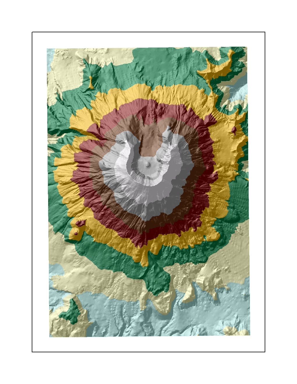
Above: Aspect spatial view with base layer.


Above: ArcScene view with lookout point.

Spatial Analysis

1. How many counties does the State of Iowa contain?
Iowa contains 99 counties.

2. Which county in Georgia contains the largest number of people, as of the year 2001?
The county with the largest population in the year 2001 was Fulton County, with 832,094 people.

3. How many cities, with populations greater than 15,000, are located within the State of Washington?
There are 39 cities in the state of WA with populations of 15,000 or more.

4. How many miles long are all of the interstates that are crossed by the outline of Los Angeles County?
The total length of all interstates in Los Angeles County add to a sum of 3851.13751 miles.

5. Simplify the Urban Boundaries feature class so that only the urban areas of Los Angeles County are visible. Include a screenshot of this new layer in your blog. How many acres of urban area lie within Los Angeles County?

There are 1,367,445 acres of urban area in L.A. County. I used the clip overlay function to simplify the Urban Boundaries feature class.

6. How many zip codes have their centroid in Los Angeles County?
There are 522 zip codes that have centroids located in L.A. County.

7. Create a layer displaying the provinces of Canada using the data provided to you in the Canada dataset. Save this new layer under the Canada dataset using the name Provinces. Include a screenshot of this new layer in your blog.
I used the dissolve tool to create a new feature class of all provinces.

8. Which Native American Indian Reservations lie within 75 miles of the City of Thurso in Quebec, Canada?
There are five reservations within a 75 mile zone of Thurso:
Indian Reserve, Doncaster Indian Reserve 17
Indian Reserve, Kitigan Zibi Indian Reserve
Indian Reserve, Kahnawake Indian Reserve 14
Indian Reserve, Kanesatake Indian Reserve 16
Indian Reserve, Akwesasne Indian Reserve 15

Census Maps

Above: All U.S. counties are ranked based on the concentration of self-reported ethnicity. Counties that reflect darker shading have higher concentrations of African-Americans. This data set, obtained in 1999, shows the highest levels of concentration in the Southeastern United States. Traditionally Southern states have the highest proportion of self-identified blacks, in which nearly half or more of the population is black. These states include Louisiana, Mississippi, Alabama, Georgia, South Carolina, North Carolina, Tennessee, Virginia and Maryland. While more diffuse, select counties in Florida, Michigan, Texas and California reported higher concentrations of blacks, nearly a quarter or more of the population. The breaks that the software created do not reveal the complexities of the differences in concentration between the 8.11% and 24.25% threshold and the 0.1% to 8.1% as well. This data set would be more revealing if contrasted, for example, with data from the 2010 Census.

Above: Overall, concentration levels of Asians were lower than for Blacks; this was due in part to the fact that there are fewer Asians in the total population than Blacks. In 1999, highest levels of self-reported Asians were concentrated in the West, mostly in the states of California, Oregon, Washington, Alaska and Hawaii. Select areas in the Eastern United States also had concentrated populations of Asians: the New York region appears to have higher concentrations. The threshold, again, is too general to give insight into how these concentrated areas compare to one another. The range, 17.57% to 46.04% does not represent diversity as clearly. Perhaps inserting another tier, ranging from 35% to 46.04% would have better illustrated the distinction. Other regions that had more diffuse, but significant concentrations of Asians, were Florida, Texas, Michigan, Arizona, Nevada and Wisconsin. Again, contrasting this data with more recent data would show trends not currently visible.

Above: Although somewhat ambiguous in its definition, this map reflects the distribution of respondents who identified themselves as "Some Other Race" in 1999. According to the 2000 Census, "Some Other Race" is an "other" category, reserved for self-reporting a race that is not represented by a given category within the survey. Because "Hispanic" or "Latino" is not a given category on the census (the only choices are White, Black or African American, Asian, American Indian or Alaska Native, Native Hawaiian or Pacific Islander, and some other race) this category is likely selected by people who self-identify as Latino. Within this category, there is the option to write in a race, such as Mexican, Puerto Rican, Cuban or some other self-reported race. Assuming that this is the primary group reflected in this map, the populations are concentrated in the Southwest, as well as the Northwest and Florida. The greatest concentrations (20.83% to 39.08%) are located in California, Arizona, New Mexico, Colorado and Texas. Washington, Kansas and Idaho also have a few counties that report relatively high concentrations.

Overall Map Series:

In order to compare these maps to each other- which would be possible, given that the data was all collected in the same year from the same survey- the breaks would have to be set equal to one another. As the maps are now, they only reflect concentrations of one race compared to total population, whereas if the breaks were set to match one another (in increments of 10% for example) then, it would be possible to compare concentrations of race by county nationally. These maps are only useful insofar as they show distribution at a given time period; however, these are static frames that do not reflect moving or changing patterns of dispersion. Because these maps were created in GIS, it would be possible to make them dynamic, given more data (from other years) and other variables, such as housing information or some other factor, to show other trends.

Overall Impressions of GIS:

Now that I better understand how GIS uses Excel tables, I can imagine using GIS in new ways. Prior to doing this lab, I didn't understand how I could find data on the web and harness GIS to analyze it, but after undertaking the process to find data sets, download them, edit them, upload them and join them, I feel like I understand how to use it in the future for more complex tasks.

ArcMap Projections

Above: Equidistant Map Projections preserve distance.from a given point.
Above: Equal Area Map Projections preserve area.

Above: Conformal Map Projections preserve angles.

Significance:

Map projections take a three-dimensional object, the earth which is a sphere, and project it onto a two-dimensional surface. Regardless of the method used, distortions always occur. This is why we different types of projections are used: equidistant projections preserve distance; equal area projections preserve area; and conformal projections preserve shape. No projection is perfect however, and depending upon the purpose of the map, the element that needs to be preserved must be identified. In preserving distance, often times, area and shape are sacrificed. This is true of the other two variables as well; therefore, different map projections serve specific purposes and should not be used for other purposes because they are inaccurate.

Perils:

Map projections can preserve area, shape, distance, scale or other factors. However, no map projection is perfect enough to preserve all properties. Because of this, distortion occurs. In changing the surface of the projections, different properties are preserved.

The conformal projections were the Mercator and the Gall Stereographic. The Mercator uses a cylindrical projection and is often used for navigation because it preserves linear scale and angle. However, it distorts shape and makes large objects seem larger than they are; the scale increases towards the poles. This is why Russia and Greenland, for example, appear inordinately large. The estimation of distance was inaccurate: standard error (the difference between the true value and the estimate divided by the true value and the result multiplied by 100) was 45.9%. The Gall Stereographic however, was far more accurate, with only 3.2% error. It projects the sphere onto a plane; it does not preserve angles, nor distances or areas of figures. It does preserve angles.

The equal area map projections were the Sinusoidal and the Mollweide. The Sinusoidal uses a pseudocylindrical projection to preserve scale along the Meridian. Area is preserved on the map. The error for the Sinusoidal projection was 16.9%. The Mollweide is also a pseudocylindrical projection that is often used to model the sky. It does not preserve angles or shape, only area. This is reflected in the curvature of the continents. Error for the Mollweide was 14.4%.

The equidistant projections were the Equidistant Conic and the Plate Caree. The Equidistant Conic is projected onto a cone and has equally spaced parallels. Area and angles are not preserved, only distances. Distortion increases below the equator. Error for the conic is 0.61%. The Plate Caree projection is a simple grid that spaces meridians and horizontals by circles of latitude. This map is highly inaccurate, but useful for thematic mapping, due to easy translation to pixels. The projection appears to be highly distorted horizontally; error is 46.8%.

Potential:

In representing distance from D.C. to Kabul, the most accurate map projection was the Equidistant Conic; it had the lowest value for standard error. The most inaccurate map projection was the Plate Caree, which had the highest error. If the time is not taken to make these comparisons among maps, reported data, such as distances, angles and area can be highly inaccurate. It is important to use projections that will best represent the properties studied.

Completed Arc Map Tutorial

Above: Exercises 1-5 of the Arc Maps tutorial.

Working hands-on, independently with the GIS software was the best way to tackle the challenge. I feel that after hearing so much about the power and potential of GIS to solve problems, there was no better way to witness this than by completing this basic tutorial. Upon reflection, I still feel that had it not been for the detailed, step by step instructions, I would have been very lost working alone, even during my second time of repeating the process. I think that this is due in part to my lack of solid computer skills and fundamental understanding about concepts such as folder hierarchies and saving my work. I have always thought of myself as a computer-literate person, but I now realize how much more I need to understand about harnessing the power of the computer in order to attack problems and manipulate data to produce logical results.

The struggles that I faced were not unlike the feeling I had when I was forced to teach myself basic knowledge of Adobe Creative Suite in the course of a week. I had to learn how to manipulate images in Photoshop, blend them with scanned sketches and organize them alongside original maps that I had created in Adobe Illustrator, into a tabletop book using InDesign. I had so many unanswered questions and I realized that if I could not figure out how to work independently, I would not succeed. This is where I gained a profound understanding, and eventually appreciation, for the concept of layers in a document. This was not unlike ArcGIS, although the data layers in GIS are more complex.

One fear that I have upon completing the tutorial comes from the realization that all of the data that I used was prefabricated and came from a reliable database. I didn’t need to find this information myself; I simply had to access it. But I can assume that this will rarely be the case in solving future problems and I feel that my understanding of how the computer finds the data, retrieves it and stores it still is somewhat unclear to me. I am becoming aware slowly of all of the resources at our disposal. But what good will these resources do me in the future, if I am not confident in how to access them?

I am amazed at the remote access technology that allowed me to complete my assignment from outside of the lab on a Mac platform. I was proud of myself for figuring out how to access the computer lab from off-campus, following the directions that were provided. I also felt a great sense of relief and satisfaction from completing the tutorial. It was an intense process to complete all five tasks, and I felt that there was so much that could go wrong at each step, especially working outside of the network on a non-PC computer. It was difficult, admittedly, to find the motivation to close my screen filled with my completed work and begin again from scratch, pushing myself not to refer back to my notes nearly as much the second time. I did feel increased confidence, but not much.

I feel that I need to still complete the tutorial several more times before I can really internalize the necessary procedures for working with data. I was so absorbed in managing details (rescaling the page, matching the color palate to that of the example) that I am worried that I did not really grasp the deeper significance of each task. In repeating these tasks, I know that I will eventually learn to break away from my myopic, detail-oriented mindset and understand the concepts behind each step. I know that when I reach this level of confidence with the software, I would actually be able to visualize what steps I would have to take in order to solve a problem, such as creating a table from two data sets in order to plot a new graph that would explain a new relationship. Until I reach that level of comfort with the software though, I know that I will be referring back to the directions from the PDF as my crutch to assist me when I become confused.

Overall, I believe that completing this tutorial helped me gain a deeper understanding of how ArcGIS can be used to solve complex problems. I had a vague understanding beforehand, but nothing makes more sense than actually attempting it individually, hands-on. Learning in this way is tough and frustrating, but as long as I keep retrying the tutorial, I believe that I will be less likely to forget how to use the software.

L.A. Neighborhoods (On A Budget): by Sara

View L.A. Neighborhoods (On A Budget): by Sara Lafia in a larger map

Potential:

In working with Google Maps, I realized the power that the digital mapmaker has. Using this technology was empowering; when I first realized what I could do with the map, I was overwhelmed with ideas. After watching the few introductory videos that were provided and skimming through some blogs, I was ready to make my map. Or was I? The learning curve was not nearly as steep as I had anticipated. I knew that I had the potential to show users the geographical context for a topic of my choice. I really wanted to come up with a way to show layers of metropolitan expansion and urban encroachment by decade through the San Fernando Valley and the Antelope Valley as well as expanding commuter routes and congestion, but I realized that I would need tools far more powerful than Google Maps to create this kind of a dynamic map. I then settled on the idea of mapping out neighborhoods within L.A. and showing sites within the areas that related to the city’s history and culture with one common theme: all activities would be free. This was possible using Google Maps. I had to compile a list of places and use the map to locate them; then I grouped them according to my own impressions and assumptions about neighborhoods. I wrote descriptions and histories of the places, and defined my own boundaries, ones that I thought coincided with the activities. The most common boundary, I decided, was the freeway, which dissected neighborhoods. Once this was done, I added links to other websites, hopefully reliable, and attached video to several locations where I thought a visual image might be helpful (time-lapse excavation at the La Brea Tar Pits, for example). I tried to include a picture with each point as well. So far, my first encounter with neogeography has been successful and encouraging.

Pitfalls:

Using the Google Maps interface was so simple, yet I reached an impasse, at which, I realized that I was also limited by its simplicity. It is useful to convey simple ideas and to show concepts such as proximity or routes, but the idea of creating layers like in GIS was difficult to imagine. In a way, linking photos and websites to my places was like creating layers, but in a completely different sense. Rather than layers of data, I was compiling layers of other peoples’ perceptions, including my own. What I created was very subjective. What if the information that I gathered was inaccurate? Because I made a map of free things to do in Los Angeles, what if I had misinterpreted my sources and misguided my users? Also, in connecting websites, such as the link to Amoeba Records, was I advertising for the company? All I was trying to do was create a map for inexpensive fun, but in doing so, was I bringing together elements that would never otherwise be linked? And did I have the authority and expertise to do this?

Consequences:

What I learned from this experience was how to create a map that I would consider sharing with my friends and family for personal use. I experimented by posting my URL on Facebook and waiting to see the reactions come in. All of my feedback so far has been positive. People seem to be impressed with the resource and a lot of my friends have said that they would consider using my map; college students love inexpensive fun! But I do not believe that it should serve as more than this. It is only a general concept, even a point of reference, that I hope could encourage other people to think of free fun. I can imagine this kind of information spreading by word of mouth and becoming convoluted and confusing as it is passed around. However, I would undoubtedly be curious if I saw a similar map for a new area that I had never explored. I would like to learn how to improve my map, since it could be a good tool in the current economy.

Beverly Hills Quadrangle Assignment

1. What is the name of the quadrangle?

It is called the Beverly Hills Quadrangle. This information is located in the upper right corner of the map.

2. What are the names of the adjacent quadrangles?

To the north is (2) the Van Nuys Quad, to the east is (5) the Hollywood Quad, to the south is (7) the Venice Quad and to the west is (4) the Topanga Quad. The northeast is (3) Burbank, to the southeast is (8) Inglewood, to the southwest is (6) an unassigned area, possibly the ocean, and to the northwest is (1) the Canoga Park Quad.

3. When was the quadrangle first created?

All data used to create the map was obtained earlier, but compiled in 1995 to create this particular quadrangle. I found this information in the lower left corner of the map.

4. What datum was used to create your map?

The datum is from the North American Datum of 1927, as well as the North American Datum of 1983. Additional datum was gathered from USGS topography from 1966, planimetry from 1978 and other sources. Hydrographic data is compiled from NOS/NOAA chart from 1964. Coordinates are from the California Coordinate System and the National Geodetic Vertical Data. This information was also from the lower left corner.

5. What is the scale of the map?

The scale is denoted in a dimensionless ratio of 1:24 000. This is found in the center at the bottom of the map.

6. At the above scale, answer the following:

a) 5 centimeters on the map is equivalent to how many meters on the ground?

5 centimeters is 1200 meters.

b) 5 inches on the map is equivalent to how many miles on the ground?

5 inches is 1.89 miles.

c) one mile on the ground is equivalent to how many inches on the map?

1 mile is 2.64 inches.

d) three kilometers on the ground is equivalent to how many centimeters on the map?

3 kilometers is 12.5 centimeters.

7. What is the contour interval on your map?

The contour interval of the map is 20 feet. The supplementary contour interval is 10 feet. This is found below the scale and graphic.

8. What are the approximate geographic coordinates in both degrees/minutes/seconds and decimal degrees of:

a) the Public Affairs Building?

DMS: 34º04'26" and -118º26'21"

DD: 34.07398º and -118.43923º

b) the tip of Santa Monica pier?

DMS: 34º0'26" and -118º30'3"

DD: 34.00732º and -118.50073º

c) the Upper Franklin Canyon Reservoir?

DMS: 34º7'18" and 118º25'33"

DD: 34.12175º and -118.40907º

9. What is the approximate elevation in both feet and meters of:

a) Greystone Mansion (in Greystone Park)?

560 feet=170.688 meters.

b) Woodlawn Cemetery?

140 feet=42.672 meters.

c) Crestwood Hills Park?

630 feet=192.024 meters.

10. What is the UTM zone of the map?

The UTM is the Universal Transverse Mercator Grid, which divides the earth into 60 north-south zones, 6 degrees wide. The Beverly Hills Quad falls into Zone 11, which covers 120 degrees to 114 degrees; the map covers a range around 118 degrees. I found a UTM Zone Map on the USGS website.

11. What are the UTM coordinates for the lower left corner of your map?

The UTM coordinates in the lower left are 3763000 and 362000.

12. How many square meters are contained within each cell (square) of the UTM gridlines?

Each UTM cell contains 1,000,000 square meters.

13. Obtain elevation measurements, from west to east along the UTM northing 3771000, where the eastings of the UTM grid intersect the northing. Create an elevation profile using these measurements in Excel. Figure out how to label the elevation values to the two measurements on campus. Insert your elevation profile as a graphic in your blog.

Above: I included all elevation estimates and indicated the two elevations on campus with yellow arrows and a label.

14. What is the magnetic declination of the map?

The declination is the difference between true north and magnetic north, so it is positive 14 degrees to the East. This is indicated by a chart at the bottom of the map.

15. In which direction does water flow in the intermittent stream between the 405 freeway and Stone Canyon Reservoir?

This stream flows from North to South.

16. Crop out (i.e., cut and paste) UCLA from the map and include it as a graphic on your blog.

Above: I included part of the Ronald Reagan Medical Center, because I wasn't sure if this would also be considered part of the UCLA campus.